The modelsum function

Introduction

Very often we are asked to summarize model results from multiple fits into a nice table. The endpoint might be of different types (e.g., survival, case/control, continuous) and there may be several independent variables that we want to examine univariately or adjusted for certain variables such as age and sex. Locally at Mayo, the SAS macros %modelsum, %glmuniv, and %logisuni were written to create such summary tables. With the increasing interest in R, we have developed the function modelsum to create similar tables within the R environment.

In developing the modelsum function, the goal was to bring the best features of these macros into an R function. However, the task was not simply to duplicate all the functionality, but rather to make use of R’s strengths (modeling, method dispersion, flexibility in function definition and output format) and make a tool that fits the needs of R users. Additionally, the results needed to fit within the general reproducible research framework so the tables could be displayed within an R markdown report.

This report provides step-by-step directions for using the functions associated with modelsum. All functions presented here are available within the arsenal package. An assumption is made that users are somewhat familiar with R markdown documents. For those who are new to the topic, a good initial resource is available at rmarkdown.rstudio.com.

Simple Example

The first step when using the modelsum function is to load the arsenal package. All the examples in this report use a dataset called mockstudy made available by Paul Novotny which includes a variety of types of variables (character, numeric, factor, ordered factor, survival) to use as examples.

> require(arsenal)
Loading required package: arsenal
> data(mockstudy) # load data
> dim(mockstudy)  # look at how many subjects and variables are in the dataset 
[1] 1499   14
> # help(mockstudy) # learn more about the dataset and variables
> str(mockstudy) # quick look at the data
'data.frame':   1499 obs. of  14 variables:
 $ case       : int  110754 99706 105271 105001 112263 86205 99508 90158 88989 90515 ...
 $ age        : int  67 74 50 71 69 56 50 57 51 63 ...
  ..- attr(*, "label")= chr "Age in Years"
 $ arm        : chr  "F: FOLFOX" "A: IFL" "A: IFL" "G: IROX" ...
  ..- attr(*, "label")= chr "Treatment Arm"
 $ sex        : Factor w/ 2 levels "Male","Female": 1 2 2 2 2 1 1 1 2 1 ...
 $ race       : chr  "Caucasian" "Caucasian" "Caucasian" "Caucasian" ...
  ..- attr(*, "label")= chr "Race"
 $ fu.time    : int  922 270 175 128 233 120 369 421 387 363 ...
 $ fu.stat    : int  2 2 2 2 2 2 2 2 2 2 ...
 $ ps         : int  0 1 1 1 0 0 0 0 1 1 ...
 $ hgb        : num  11.5 10.7 11.1 12.6 13 10.2 13.3 12.1 13.8 12.1 ...
 $ bmi        : num  25.1 19.5 NA 29.4 26.4 ...
  ..- attr(*, "label")= chr "Body Mass Index (kg/m^2)"
 $ alk.phos   : int  160 290 700 771 350 569 162 152 231 492 ...
 $ ast        : int  35 52 100 68 35 27 16 12 25 18 ...
 $ mdquality.s: int  NA 1 1 1 NA 1 1 1 1 1 ...
 $ age.ord    : Ord.factor w/ 8 levels "10-19"<"20-29"<..: 6 7 4 7 6 5 4 5 5 6 ...

To create a simple linear regression table (the default), use a formula statement to specify the variables that you want summarized. The example below predicts BMI with the variables sex and age.

> tab1 <- modelsum(bmi ~ sex + age, data=mockstudy)

If you want to take a quick look at the table, you can use summary on your modelsum object and the table will print out as text in your R console window. If you use summary without any options you will see a number of $\ $ statements which translates to “space” in HTML.

Pretty text version of table

If you want a nicer version in your console window then adding the text=TRUE option.

> summary(tab1, text=TRUE)


|             |estimate |std.error |p.value |adj.r.squared |Nmiss |
|:------------|:--------|:---------|:-------|:-------------|:-----|
|(Intercept)  |27.491   |0.181     |< 0.001 |0.004         |33    |
|sex Female   |-0.731   |0.290     |0.012   |              |      |
|(Intercept)  |26.424   |0.752     |< 0.001 |0.000         |33    |
|Age in Years |0.013    |0.012     |0.290   |              |      |

Pretty Rmarkdown version of table

In order for the report to look nice within an R markdown (knitr) report, you just need to specify results="asis" when creating the r chunk. This changes the layout slightly (compresses it) and bolds the variable names.

> summary(tab1)

	estimate	std.error	p.value	adj.r.squared	Nmiss
(Intercept)	27.491	0.181	< 0.001	0.004	33
sex Female	-0.731	0.290	0.012
(Intercept)	26.424	0.752	< 0.001	0.000	33
Age in Years	0.013	0.012	0.290

Data frame version of table

If you want a data.frame version, simply use as.data.frame.

> as.data.frame(tab1)
  y.term                  y.label strata.term adjustment model        term
1    bmi Body Mass Index (kg/m^2)             unadjusted     1 (Intercept)
2    bmi Body Mass Index (kg/m^2)             unadjusted     1   sexFemale
3    bmi Body Mass Index (kg/m^2)             unadjusted     2 (Intercept)
4    bmi Body Mass Index (kg/m^2)             unadjusted     2         age
         label term.type    estimate  std.error       p.value adj.r.squared
1  (Intercept) Intercept 27.49147713 0.18134740  0.000000e+00  3.632258e-03
2   sex Female      Term -0.73105055 0.29032223  1.190605e-02  3.632258e-03
3  (Intercept) Intercept 26.42372272 0.75211474 1.279109e-196  8.354809e-05
4 Age in Years      Term  0.01304859 0.01231653  2.895753e-01  8.354809e-05
  Nmiss
1    33
2    33
3    33
4    33

Add an adjustor to the model

The argument adjust allows the user to indicate that all the variables should be adjusted for these terms. To adjust each model for age and sex (for instance), we use adjust = ~ age + sex:

> tab2 <- modelsum(alk.phos ~ arm + ps + hgb, adjust= ~age + sex, data=mockstudy)
> summary(tab2)

	estimate	std.error	p.value	adj.r.squared	Nmiss
(Intercept)	175.548	20.587	< 0.001	-0.001	266
Treatment Arm F: FOLFOX	-13.701	8.730	0.117
Treatment Arm G: IROX	-2.245	9.860	0.820
Age in Years	-0.017	0.319	0.956
sex Female	3.016	7.521	0.688
(Intercept)	148.391	19.585	< 0.001	0.045	266
ps	46.721	5.987	< 0.001
Age in Years	-0.084	0.311	0.787
sex Female	1.169	7.343	0.874
(Intercept)	336.554	32.239	< 0.001	0.031	266
hgb	-13.845	2.137	< 0.001
Age in Years	0.095	0.314	0.763
sex Female	-5.980	7.516	0.426

Models for each endpoint type

To make sure the correct model is run you need to specify “family”. The options available right now are : gaussian, binomial, survival, and poisson. If there is enough interest, additional models can be added.

Gaussian

Fit and summarize linear regression model

Look at whether there is any evidence that AlkPhos values vary by study arm after adjusting for sex and age (assuming a linear age relationship).

> fit <- lm(alk.phos ~ arm + age + sex, data=mockstudy)
> summary(fit)

Call:
lm(formula = alk.phos ~ arm + age + sex, data = mockstudy)

Residuals:
    Min      1Q  Median      3Q     Max 
-168.80  -81.45  -47.17   37.39  853.56 

Coefficients:
              Estimate Std. Error t value Pr(>|t|)    
(Intercept)  175.54808   20.58665   8.527   <2e-16 ***
armF: FOLFOX -13.70062    8.72963  -1.569    0.117    
armG: IROX    -2.24498    9.86004  -0.228    0.820    
age           -0.01741    0.31878  -0.055    0.956    
sexFemale      3.01598    7.52097   0.401    0.688    
---
Signif. codes:  0 '***' 0.001 '**' 0.01 '*' 0.05 '.' 0.1 ' ' 1

Residual standard error: 128.5 on 1228 degrees of freedom
  (266 observations deleted due to missingness)
Multiple R-squared:  0.002552,  Adjusted R-squared:  -0.0006969 
F-statistic: 0.7855 on 4 and 1228 DF,  p-value: 0.5346
> plot(fit)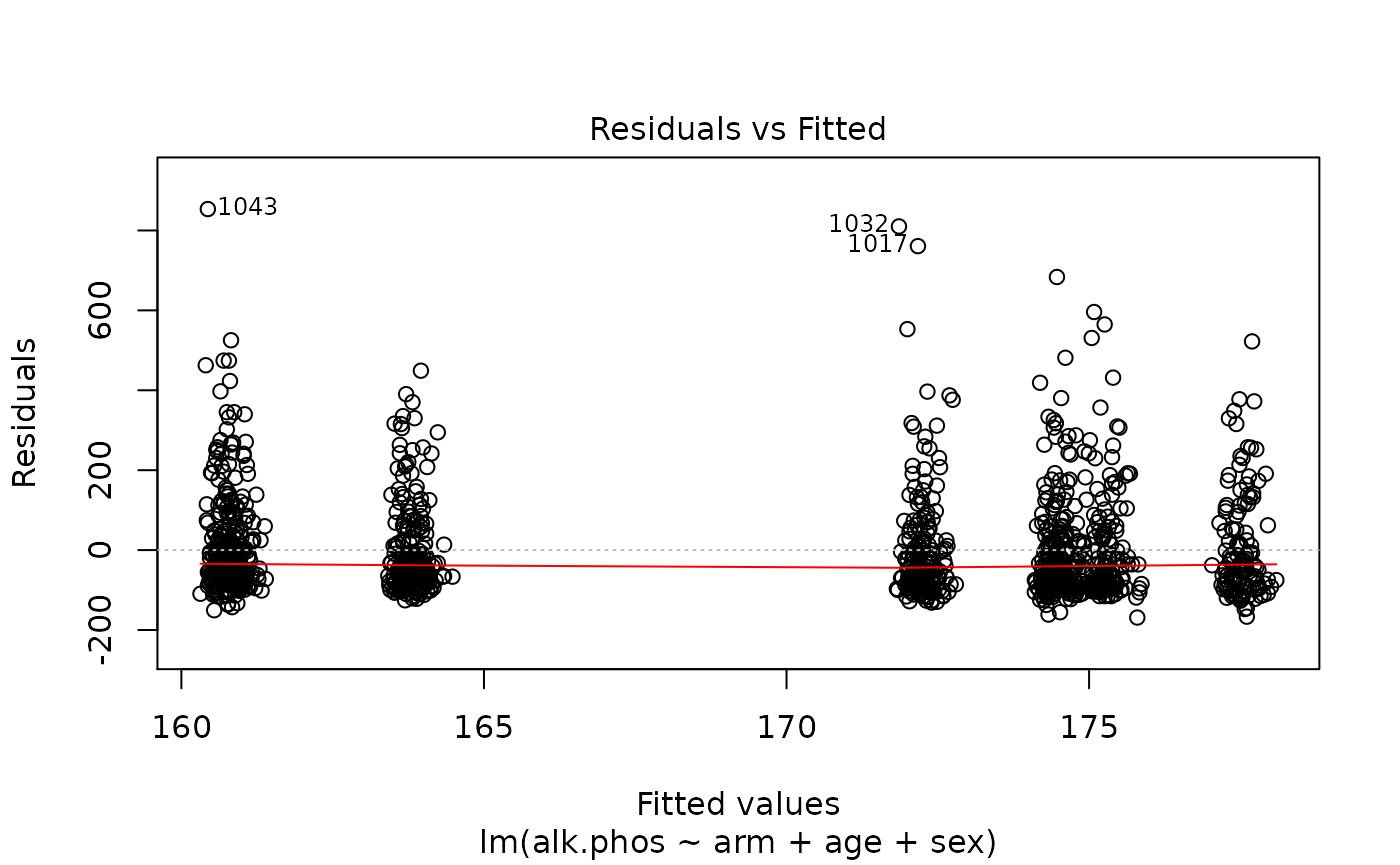

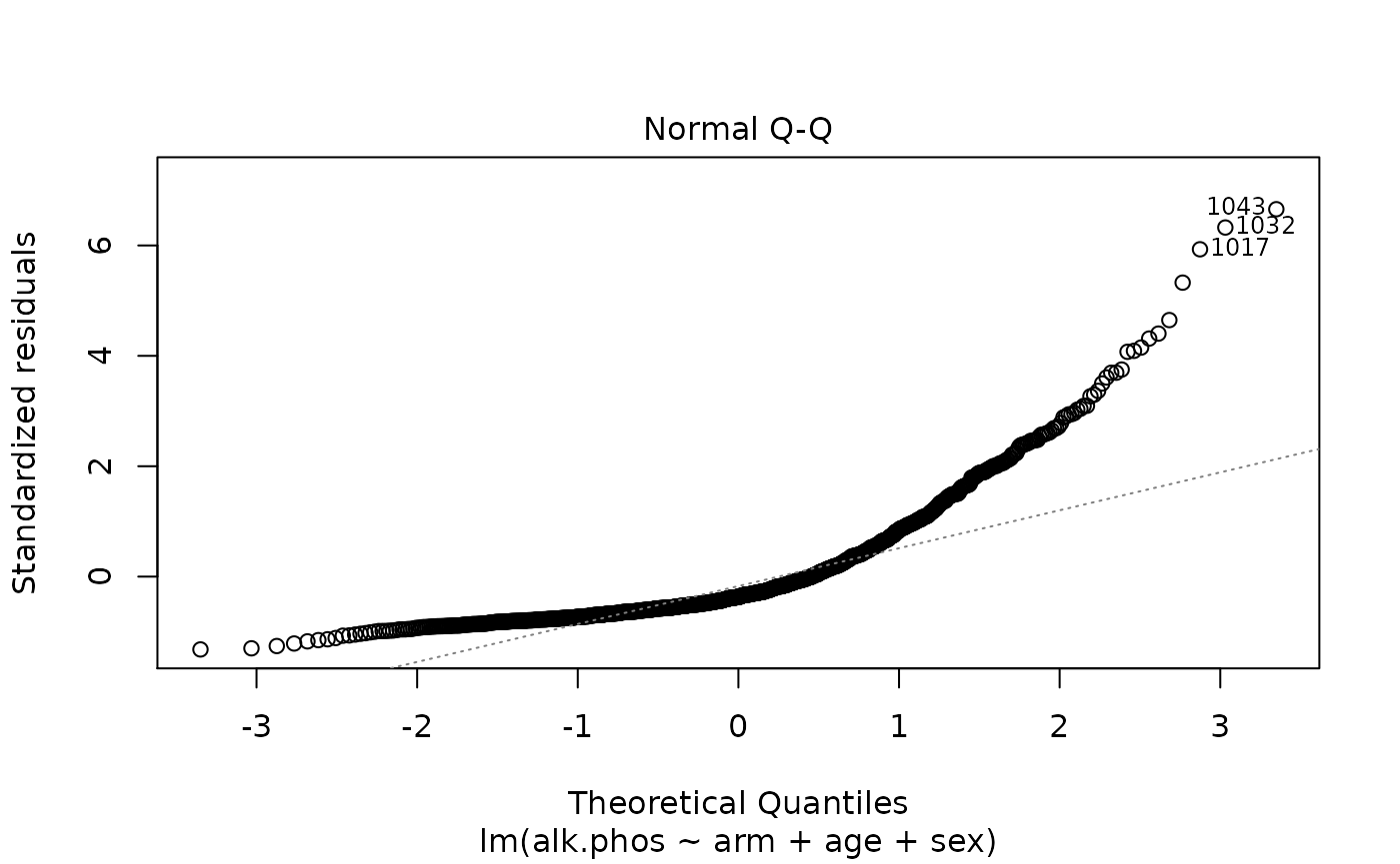
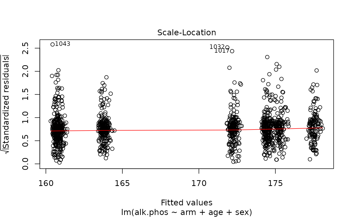
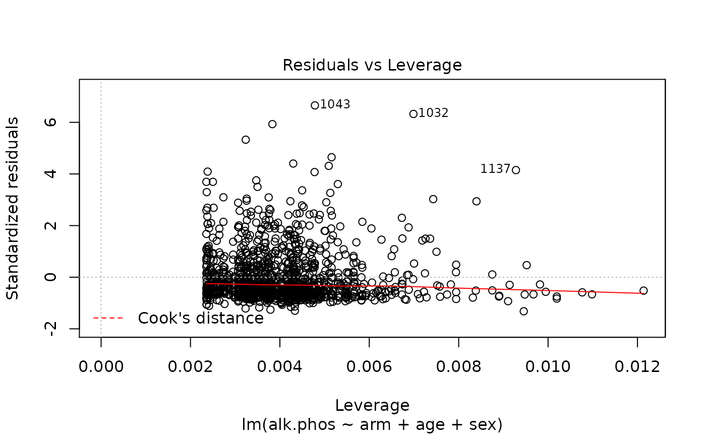
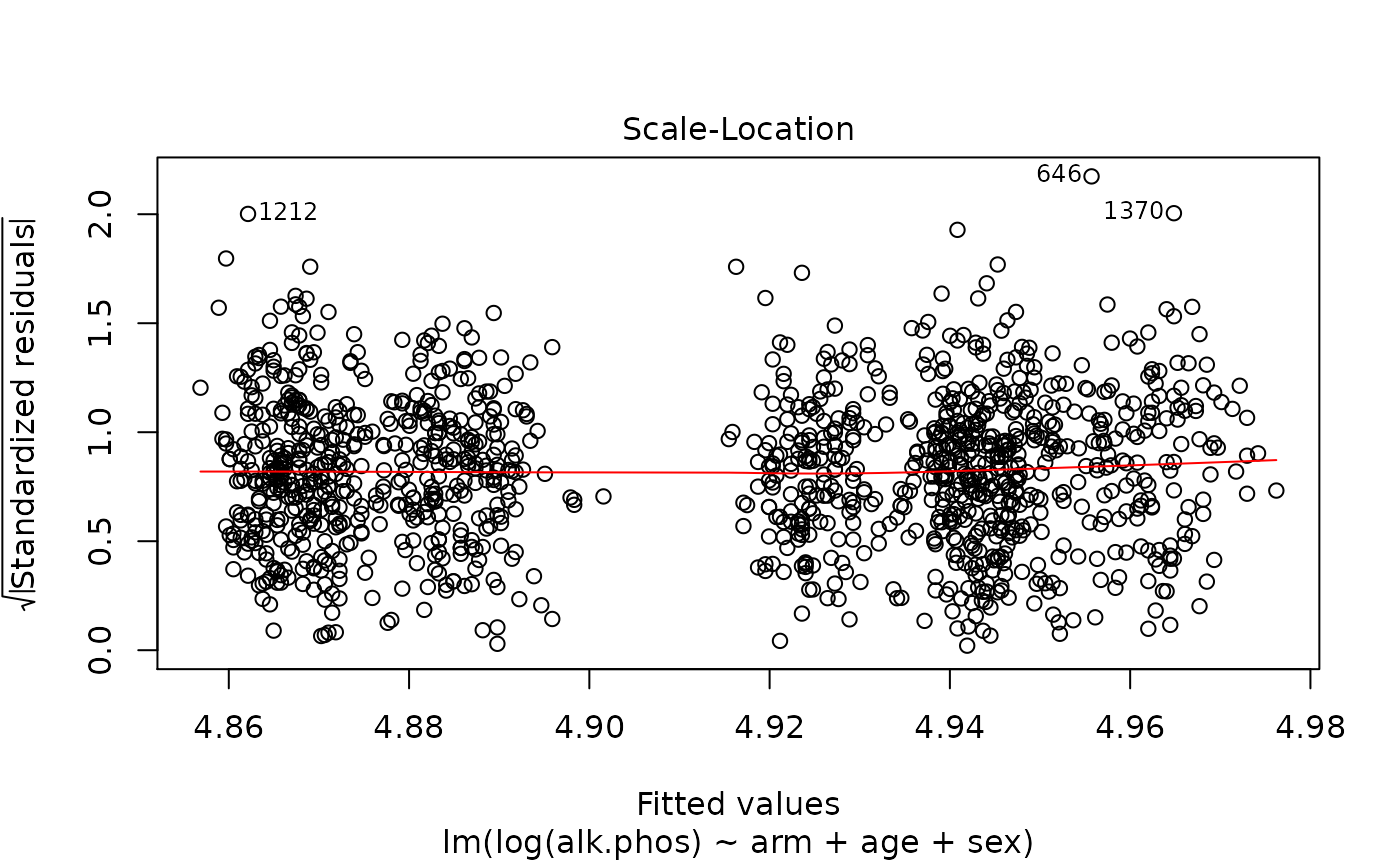
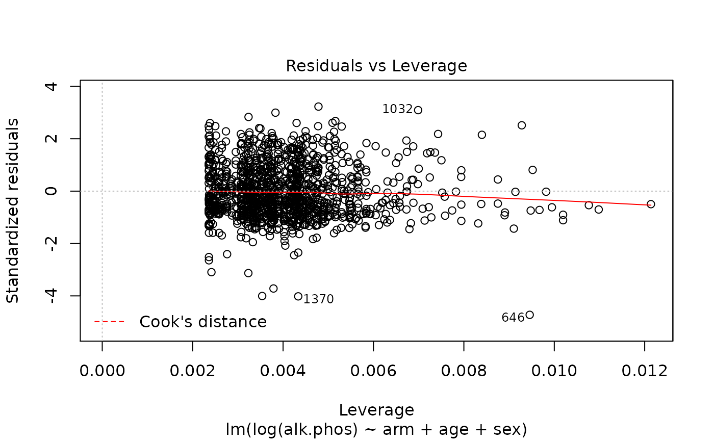
The results suggest that the endpoint may need to be transformed. Calculating the Box-Cox transformation suggests a log transformation.

> require(MASS)
> boxcox(fit)

> fit2 <- lm(log(alk.phos) ~ arm + age + sex, data=mockstudy)
> summary(fit2)

Call:
lm(formula = log(alk.phos) ~ arm + age + sex, data = mockstudy)

Residuals:
    Min      1Q  Median      3Q     Max 
-3.0098 -0.4470 -0.1065  0.4205  2.0620 

Coefficients:
               Estimate Std. Error t value Pr(>|t|)    
(Intercept)   4.9692474  0.1025239  48.469   <2e-16 ***
armF: FOLFOX -0.0766798  0.0434746  -1.764    0.078 .  
armG: IROX   -0.0192828  0.0491041  -0.393    0.695    
age          -0.0004058  0.0015876  -0.256    0.798    
sexFemale     0.0179253  0.0374553   0.479    0.632    
---
Signif. codes:  0 '***' 0.001 '**' 0.01 '*' 0.05 '.' 0.1 ' ' 1

Residual standard error: 0.6401 on 1228 degrees of freedom
  (266 observations deleted due to missingness)
Multiple R-squared:  0.003121,  Adjusted R-squared:  -0.0001258 
F-statistic: 0.9613 on 4 and 1228 DF,  p-value: 0.4278
> plot(fit2)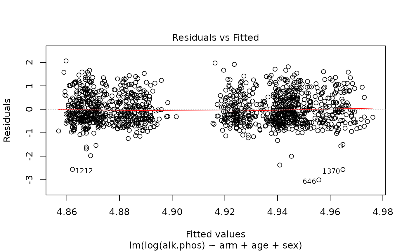

Finally, look to see whether there there is a non-linear relationship with age.

> require(splines)
Loading required package: splines
> fit3 <- lm(log(alk.phos) ~ arm + ns(age, df=2) + sex, data=mockstudy)
> 
> # test whether there is a difference between models 
> stats::anova(fit2,fit3)
Analysis of Variance Table

Model 1: log(alk.phos) ~ arm + age + sex
Model 2: log(alk.phos) ~ arm + ns(age, df = 2) + sex
  Res.Df    RSS Df Sum of Sq      F  Pr(>F)  
1   1228 503.19                              
2   1227 502.07  1    1.1137 2.7218 0.09924 .
---
Signif. codes:  0 '***' 0.001 '**' 0.01 '*' 0.05 '.' 0.1 ' ' 1
> 
> # look at functional form of age
> termplot(fit3, term=2, se=T, rug=T)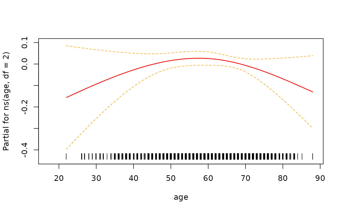

In this instance it looks like there isn’t enough evidence to say that the relationship is non-linear.

Extract data using the `broom` package

The broom package makes it easy to extract information from the fit.

> tmp <- tidy(fit3) # coefficients, p-values
> class(tmp)
[1] "tbl_df"     "tbl"        "data.frame"
> tmp
 [38;5;246m# A tibble: 6 × 5 [39m
  term             estimate std.error statistic   p.value
   [3m [38;5;246m<chr> [39m [23m                [3m [38;5;246m<dbl> [39m [23m      [3m [38;5;246m<dbl> [39m [23m      [3m [38;5;246m<dbl> [39m [23m      [3m [38;5;246m<dbl> [39m [23m
 [38;5;250m1 [39m (Intercept)        4.76      0.141     33.8   1.93 [38;5;246me [39m [31m-177 [39m
 [38;5;250m2 [39m armF: FOLFOX      - [31m0 [39m [31m. [39m [31m0 [39m [31m76 [4m7 [24m [39m    0.043 [4m4 [24m    - [31m1 [39m [31m. [39m [31m77 [39m  7.78 [38;5;246me [39m [31m-  2 [39m
 [38;5;250m3 [39m armG: IROX        - [31m0 [39m [31m. [39m [31m0 [39m [31m19 [4m5 [24m [39m    0.049 [4m1 [24m    - [31m0 [39m [31m. [39m [31m396 [39m 6.92 [38;5;246me [39m [31m-  1 [39m
 [38;5;250m4 [39m ns(age, df = 2)1   0.330     0.260      1.27  2.04 [38;5;246me [39m [31m-  1 [39m
 [38;5;250m5 [39m ns(age, df = 2)2  - [31m0 [39m [31m. [39m [31m101 [39m     0.093 [4m5 [24m    - [31m1 [39m [31m. [39m [31m0 [39m [31m8 [39m  2.82 [38;5;246me [39m [31m-  1 [39m
 [38;5;250m6 [39m sexFemale          0.018 [4m3 [24m    0.037 [4m4 [24m     0.489 6.25 [38;5;246me [39m [31m-  1 [39m
> 
> glance(fit3)
 [38;5;246m# A tibble: 1 × 12 [39m
  r.squared adj.r.squared sigma statistic p.value    df logLik   AIC   BIC
       [3m [38;5;246m<dbl> [39m [23m          [3m [38;5;246m<dbl> [39m [23m  [3m [38;5;246m<dbl> [39m [23m      [3m [38;5;246m<dbl> [39m [23m    [3m [38;5;246m<dbl> [39m [23m  [3m [38;5;246m<dbl> [39m [23m   [3m [38;5;246m<dbl> [39m [23m  [3m [38;5;246m<dbl> [39m [23m  [3m [38;5;246m<dbl> [39m [23m
 [38;5;250m1 [39m   0.005 [4m3 [24m [4m3 [24m       0.001 [4m2 [24m [4m7 [24m 0.640      1.31   0.255     5 - [31m [4m1 [24m19 [39m [31m6 [39m [31m. [39m  [4m2 [24m405.  [4m2 [24m441.
 [38;5;246m# ℹ 3 more variables: deviance <dbl>, df.residual <int>, nobs <int> [39m

Create a summary table using modelsum

> ms.logy <- modelsum(log(alk.phos) ~ arm + ps + hgb, data=mockstudy, adjust= ~age + sex, 
+                     family=gaussian,  
+                     gaussian.stats=c("estimate","CI.lower.estimate","CI.upper.estimate","p.value"))
> summary(ms.logy)

	estimate	CI.lower.estimate	CI.upper.estimate	p.value
(Intercept)	4.969	4.768	5.170	< 0.001
Treatment Arm F: FOLFOX	-0.077	-0.162	0.009	0.078
Treatment Arm G: IROX	-0.019	-0.116	0.077	0.695
Age in Years	-0.000	-0.004	0.003	0.798
sex Female	0.018	-0.056	0.091	0.632
(Intercept)	4.832	4.640	5.023	< 0.001
ps	0.226	0.167	0.284	< 0.001
Age in Years	-0.001	-0.004	0.002	0.636
sex Female	0.009	-0.063	0.081	0.814
(Intercept)	5.765	5.450	6.080	< 0.001
hgb	-0.069	-0.090	-0.048	< 0.001
Age in Years	0.000	-0.003	0.003	0.925
sex Female	-0.027	-0.101	0.046	0.468

Binomial

Fit and summarize logistic regression model

> boxplot(age ~ mdquality.s, data=mockstudy, ylab=attr(mockstudy$age,'label'), xlab='mdquality.s')

> 
> fit <- glm(mdquality.s ~ age + sex, data=mockstudy, family=binomial)
> summary(fit)

Call:
glm(formula = mdquality.s ~ age + sex, family = binomial, data = mockstudy)

Coefficients:
             Estimate Std. Error z value Pr(>|z|)    
(Intercept)  2.329442   0.514684   4.526 6.01e-06 ***
age         -0.002353   0.008256  -0.285    0.776    
sexFemale    0.039227   0.195330   0.201    0.841    
---
Signif. codes:  0 '***' 0.001 '**' 0.01 '*' 0.05 '.' 0.1 ' ' 1

(Dispersion parameter for binomial family taken to be 1)

    Null deviance: 807.68  on 1246  degrees of freedom
Residual deviance: 807.55  on 1244  degrees of freedom
  (252 observations deleted due to missingness)
AIC: 813.55

Number of Fisher Scoring iterations: 4
> 
> # create Odd's ratio w/ confidence intervals
> tmp <- data.frame(summary(fit)$coef)
> tmp
                Estimate  Std..Error    z.value     Pr...z..
(Intercept)  2.329441734 0.514683688  4.5259677 6.011977e-06
age         -0.002353404 0.008255814 -0.2850602 7.755980e-01
sexFemale    0.039227292 0.195330166  0.2008256 8.408350e-01
> 
> tmp$OR <- round(exp(tmp[,1]),2)
> tmp$lower.CI <- round(exp(tmp[,1] - 1.96* tmp[,2]),2)
> tmp$upper.CI <- round(exp(tmp[,1] + 1.96* tmp[,2]),2)
> names(tmp)[4] <- 'P-value'
> 
> kable(tmp[,c('OR','lower.CI','upper.CI','P-value')])

	OR	lower.CI	upper.CI	P-value
(Intercept)	10.27	3.75	28.17	0.000006
age	1.00	0.98	1.01	0.775598
sexFemale	1.04	0.71	1.53	0.840835

> 
> # Assess the predictive ability of the model
> 
> # code using the pROC package
> require(pROC)
> pred <- predict(fit, type='response')
> tmp <- pROC::roc(mockstudy$mdquality.s[!is.na(mockstudy$mdquality.s)]~ pred, plot=TRUE, percent=TRUE)
Setting levels: control = 0, case = 1
Setting direction: controls < cases

> tmp$auc
Area under the curve: 50.69%

Extract data using `broom` package

The broom package makes it easy to extract information from the fit.

> tidy(fit, exp=T, conf.int=T) # coefficients, p-values, conf.intervals
 [38;5;246m# A tibble: 3 × 7 [39m
  term        estimate std.error statistic    p.value conf.low conf.high
   [3m [38;5;246m<chr> [39m [23m           [3m [38;5;246m<dbl> [39m [23m      [3m [38;5;246m<dbl> [39m [23m      [3m [38;5;246m<dbl> [39m [23m       [3m [38;5;246m<dbl> [39m [23m     [3m [38;5;246m<dbl> [39m [23m      [3m [38;5;246m<dbl> [39m [23m
 [38;5;250m1 [39m (Intercept)   10.3     0.515       4.53  0.000 [4m0 [24m [4m0 [24m [4m6 [24m01    3.83      28.9 
 [38;5;250m2 [39m age            0.998   0.008 [4m2 [24m [4m6 [24m    - [31m0 [39m [31m. [39m [31m285 [39m 0.776         0.981      1.01
 [38;5;250m3 [39m sexFemale      1.04    0.195       0.201 0.841         0.712      1.53
> 
> glance(fit) # model summary statistics
 [38;5;246m# A tibble: 1 × 8 [39m
  null.deviance df.null logLik   AIC   BIC deviance df.residual  nobs
           [3m [38;5;246m<dbl> [39m [23m    [3m [38;5;246m<int> [39m [23m   [3m [38;5;246m<dbl> [39m [23m  [3m [38;5;246m<dbl> [39m [23m  [3m [38;5;246m<dbl> [39m [23m     [3m [38;5;246m<dbl> [39m [23m        [3m [38;5;246m<int> [39m [23m  [3m [38;5;246m<int> [39m [23m
 [38;5;250m1 [39m          808.     [4m1 [24m246  - [31m404 [39m [31m. [39m  814.  829.     808.         [4m1 [24m244   [4m1 [24m247

Create a summary table using modelsum

> summary(modelsum(mdquality.s ~ age + bmi, data=mockstudy, adjust=~sex, family=binomial))

	OR	CI.lower.OR	CI.upper.OR	p.value	concordance	Nmiss
(Intercept)	10.272	3.831	28.876	< 0.001	0.507	252
Age in Years	0.998	0.981	1.014	0.776
sex Female	1.040	0.712	1.534	0.841
(Intercept)	4.814	1.709	13.221	0.003	0.550	273
Body Mass Index (kg/m^2)	1.023	0.987	1.063	0.220
sex Female	1.053	0.717	1.561	0.794

> 
> fitall <- modelsum(mdquality.s ~ age, data=mockstudy, family=binomial,
+                    binomial.stats=c("Nmiss2","OR","p.value"))
> summary(fitall)

	OR	p.value	Nmiss2
(Intercept)	10.493	< 0.001	252
Age in Years	0.998	0.766

Survival

Fit and summarize a Cox regression model

> require(survival)
Loading required package: survival
> 
> # multivariable model with all 3 terms
> fit  <- coxph(Surv(fu.time, fu.stat) ~ age + sex + arm, data=mockstudy)
> summary(fit)
Call:
coxph(formula = Surv(fu.time, fu.stat) ~ age + sex + arm, data = mockstudy)

  n= 1499, number of events= 1356 

                  coef exp(coef)  se(coef)      z Pr(>|z|)    
age           0.004600  1.004611  0.002501  1.839   0.0659 .  
sexFemale     0.039893  1.040699  0.056039  0.712   0.4765    
armF: FOLFOX -0.454650  0.634670  0.064878 -7.008 2.42e-12 ***
armG: IROX   -0.140785  0.868676  0.072760 -1.935   0.0530 .  
---
Signif. codes:  0 '***' 0.001 '**' 0.01 '*' 0.05 '.' 0.1 ' ' 1

             exp(coef) exp(-coef) lower .95 upper .95
age             1.0046     0.9954    0.9997    1.0095
sexFemale       1.0407     0.9609    0.9324    1.1615
armF: FOLFOX    0.6347     1.5756    0.5589    0.7207
armG: IROX      0.8687     1.1512    0.7532    1.0018

Concordance= 0.563  (se = 0.009 )
Likelihood ratio test= 56.21  on 4 df,   p=2e-11
Wald test            = 56.26  on 4 df,   p=2e-11
Score (logrank) test = 56.96  on 4 df,   p=1e-11
> 
> # check proportional hazards assumption
> fit.z <- cox.zph(fit)
> fit.z
       chisq df    p
age     1.41  1 0.24
sex     1.08  1 0.30
arm     1.80  2 0.41
GLOBAL  4.68  4 0.32
> plot(fit.z[1], resid=FALSE) # makes for a cleaner picture in this case
> abline(h=coef(fit)[1], col='red')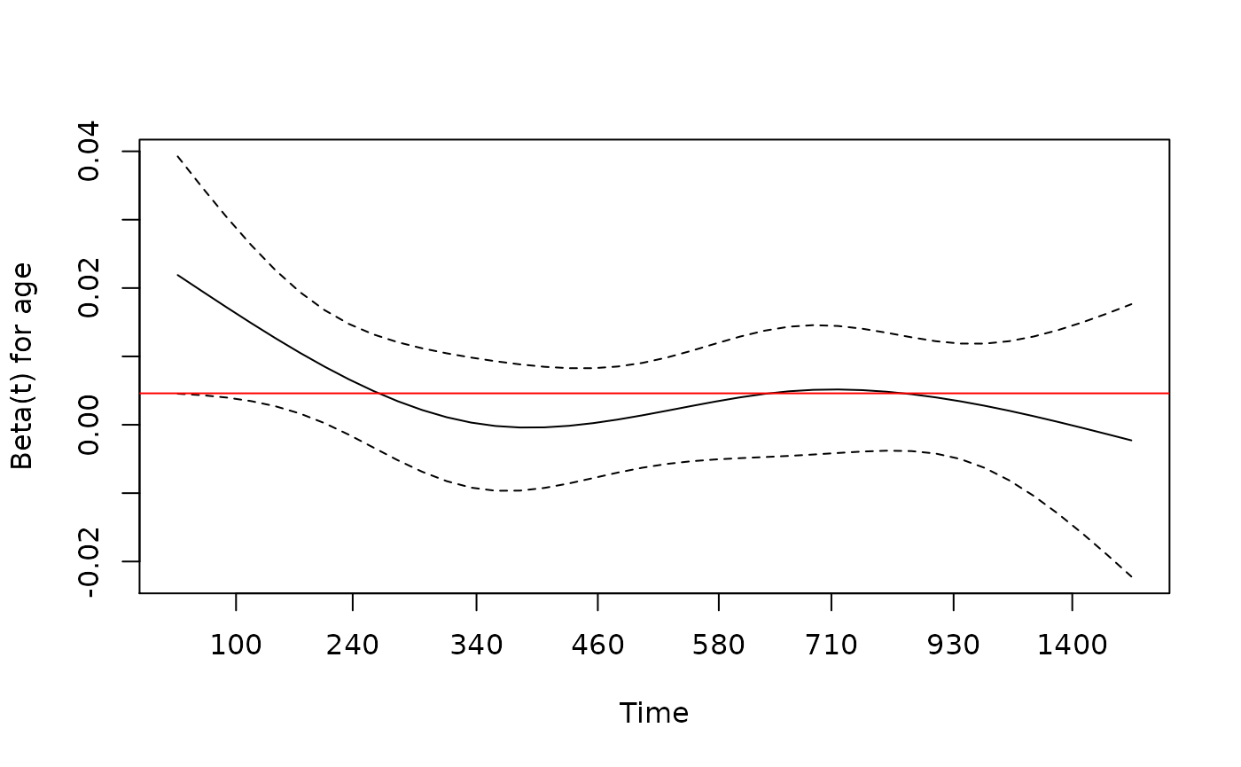

> 
> # check functional form for age using pspline (penalized spline)
> # results are returned for the linear and non-linear components
> fit2 <- coxph(Surv(fu.time, fu.stat) ~ pspline(age) + sex + arm, data=mockstudy)
> fit2
Call:
coxph(formula = Surv(fu.time, fu.stat) ~ pspline(age) + sex + 
    arm, data = mockstudy)

                         coef se(coef)      se2    Chisq   DF       p
pspline(age), linear  0.00443  0.00237  0.00237  3.48989 1.00  0.0617
pspline(age), nonlin                            13.11270 3.08  0.0047
sexFemale             0.03993  0.05610  0.05607  0.50663 1.00  0.4766
armF: FOLFOX         -0.46240  0.06494  0.06493 50.69608 1.00 1.1e-12
armG: IROX           -0.15243  0.07301  0.07299  4.35876 1.00  0.0368

Iterations: 6 outer, 16 Newton-Raphson
     Theta= 0.954 
Degrees of freedom for terms= 4.1 1.0 2.0 
Likelihood ratio test=70.1  on 7.08 df, p=2e-12
n= 1499, number of events= 1356 
> 
> # plot smoothed age to visualize why significant
> termplot(fit2, se=T, terms=1)
> abline(h=0)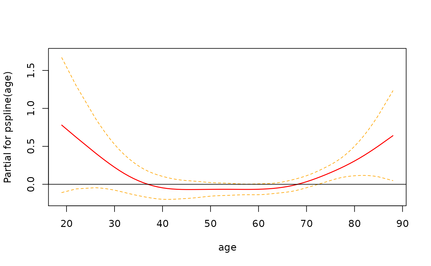

> 
> # The c-statistic comes out in the summary of the fit
> summary(fit2)$concordance
          C       se(C) 
0.568432549 0.008487495 
> 
> # It can also be calculated using the survConcordance function
> survConcordance(Surv(fu.time, fu.stat) ~ predict(fit2), data=mockstudy)
Warning in survConcordance(Surv(fu.time, fu.stat) ~ predict(fit2), data = mockstudy): 'survConcordance' is deprecated.
Use 'concordance' instead.
See help("Deprecated")
Warning in survConcordance.fit(Y, x, strat, wt): 'survConcordance.fit' is deprecated.
Use 'concordancefit' instead.
See help("Deprecated")
$concordance
concordant 
 0.5684325 

$stats
concordant discordant  tied.risk  tied.time   std(c-d) 
 620221.00  470282.00    5021.00     766.00   19235.49 

$n
[1] 1499

$std.err
   std(c-d) 
0.008779125 

$call
survConcordance(formula = Surv(fu.time, fu.stat) ~ predict(fit2), 
    data = mockstudy)

attr(,"class")
[1] "survConcordance"

Extract data using `broom` package

The broom package makes it easy to extract information from the fit.

> tidy(fit) # coefficients, p-values
 [38;5;246m# A tibble: 4 × 5 [39m
  term         estimate std.error statistic  p.value
   [3m [38;5;246m<chr> [39m [23m            [3m [38;5;246m<dbl> [39m [23m      [3m [38;5;246m<dbl> [39m [23m      [3m [38;5;246m<dbl> [39m [23m     [3m [38;5;246m<dbl> [39m [23m
 [38;5;250m1 [39m age           0.004 [4m6 [24m [4m0 [24m   0.002 [4m5 [24m [4m0 [24m     1.84  6.59 [38;5;246me [39m [31m- 2 [39m
 [38;5;250m2 [39m sexFemale     0.039 [4m9 [24m    0.056 [4m0 [24m      0.712 4.77 [38;5;246me [39m [31m- 1 [39m
 [38;5;250m3 [39m armF: FOLFOX - [31m0 [39m [31m. [39m [31m455 [39m     0.064 [4m9 [24m     - [31m7 [39m [31m. [39m [31m0 [39m [31m1 [39m  2.42 [38;5;246me [39m [31m-12 [39m
 [38;5;250m4 [39m armG: IROX   - [31m0 [39m [31m. [39m [31m141 [39m     0.072 [4m8 [24m     - [31m1 [39m [31m. [39m [31m93 [39m  5.30 [38;5;246me [39m [31m- 2 [39m
> 
> glance(fit) # model summary statistics
 [38;5;246m# A tibble: 1 × 18 [39m
      n nevent statistic.log p.value.log statistic.sc p.value.sc statistic.wald
   [3m [38;5;246m<int> [39m [23m   [3m [38;5;246m<dbl> [39m [23m          [3m [38;5;246m<dbl> [39m [23m        [3m [38;5;246m<dbl> [39m [23m         [3m [38;5;246m<dbl> [39m [23m       [3m [38;5;246m<dbl> [39m [23m           [3m [38;5;246m<dbl> [39m [23m
 [38;5;250m1 [39m   [4m1 [24m499    [4m1 [24m356          56.2    1.81 [38;5;246me [39m [31m-11 [39m         57.0   1.26 [38;5;246me [39m [31m-11 [39m           56.3
 [38;5;246m# ℹ 11 more variables: p.value.wald <dbl>, statistic.robust <dbl>, [39m
 [38;5;246m#   p.value.robust <dbl>, r.squared <dbl>, r.squared.max <dbl>, [39m
 [38;5;246m#   concordance <dbl>, std.error.concordance <dbl>, logLik <dbl>, AIC <dbl>, [39m
 [38;5;246m#   BIC <dbl>, nobs <dbl> [39m

Create a summary table using modelsum

> ##Note: You must use quotes when specifying family="survival" 
> ##      family=survival will not work
> summary(modelsum(Surv(fu.time, fu.stat) ~ arm, 
+                  adjust=~age + sex, data=mockstudy, family="survival"))

	HR	CI.lower.HR	CI.upper.HR	p.value	concordance
Treatment Arm F: FOLFOX	0.635	0.559	0.721	< 0.001	0.563
Treatment Arm G: IROX	0.869	0.753	1.002	0.053
Age in Years	1.005	1.000	1.010	0.066
sex Female	1.041	0.932	1.162	0.477

> 
> ##Note: the pspline term is not working yet
> #summary(modelsum(Surv(fu.time, fu.stat) ~ arm, 
> #                adjust=~pspline(age) + sex, data=mockstudy, family='survival'))

Poisson

Poisson regression is useful when predicting an outcome variable representing counts. It can also be useful when looking at survival data. Cox models and Poisson models are very closely related and survival data can be summarized using Poisson regression. If you have overdispersion (see if the residual deviance is much larger than degrees of freedom), you may want to use quasipoisson() instead of poisson(). Some of these diagnostics need to be done outside of modelsum.

Example 1: fit and summarize a Poisson regression model

For the first example, use the solder dataset available in the rpart package. The endpoint skips has a definite Poisson look.

> require(rpart) ##just to get access to solder dataset
> data(solder)
> hist(solder$skips)

> 
> fit <- glm(skips ~ Opening + Solder + Mask , data=solder, family=poisson)
> stats::anova(fit, test='Chi')
Analysis of Deviance Table

Model: poisson, link: log

Response: skips

Terms added sequentially (first to last)

        Df Deviance Resid. Df Resid. Dev  Pr(>Chi)    
NULL                      899     8788.2              
Opening  2   2920.5       897     5867.7 < 2.2e-16 ***
Solder   1   1168.4       896     4699.3 < 2.2e-16 ***
Mask     4   2015.7       892     2683.7 < 2.2e-16 ***
---
Signif. codes:  0 '***' 0.001 '**' 0.01 '*' 0.05 '.' 0.1 ' ' 1
> summary(fit)

Call:
glm(formula = skips ~ Opening + Solder + Mask, family = poisson, 
    data = solder)

Coefficients:
            Estimate Std. Error z value Pr(>|z|)    
(Intercept) -1.12220    0.07742  -14.50  < 2e-16 ***
OpeningM     0.57161    0.05707   10.02  < 2e-16 ***
OpeningS     1.81475    0.05044   35.98  < 2e-16 ***
SolderThin   0.84682    0.03327   25.45  < 2e-16 ***
MaskA3       0.51315    0.07098    7.23 4.83e-13 ***
MaskA6       1.81103    0.06609   27.40  < 2e-16 ***
MaskB3       1.20225    0.06697   17.95  < 2e-16 ***
MaskB6       1.86648    0.06310   29.58  < 2e-16 ***
---
Signif. codes:  0 '***' 0.001 '**' 0.01 '*' 0.05 '.' 0.1 ' ' 1

(Dispersion parameter for poisson family taken to be 1)

    Null deviance: 8788.2  on 899  degrees of freedom
Residual deviance: 2683.7  on 892  degrees of freedom
AIC: 4802.2

Number of Fisher Scoring iterations: 5

Overdispersion is when the Residual deviance is larger than the degrees of freedom. This can be tested, approximately using the following code. The goal is to have a p-value that is $>0.05$ .

> 1-pchisq(fit$deviance, fit$df.residual)
[1] 0

One possible solution is to use the quasipoisson family instead of the poisson family. This adjusts for the overdispersion.

> fit2 <- glm(skips ~ Opening + Solder + Mask, data=solder, family=quasipoisson)
> summary(fit2)

Call:
glm(formula = skips ~ Opening + Solder + Mask, family = quasipoisson, 
    data = solder)

Coefficients:
            Estimate Std. Error t value Pr(>|t|)    
(Intercept) -1.12220    0.13483  -8.323 3.19e-16 ***
OpeningM     0.57161    0.09939   5.751 1.22e-08 ***
OpeningS     1.81475    0.08784  20.660  < 2e-16 ***
SolderThin   0.84682    0.05794  14.615  < 2e-16 ***
MaskA3       0.51315    0.12361   4.151 3.62e-05 ***
MaskA6       1.81103    0.11510  15.735  < 2e-16 ***
MaskB3       1.20225    0.11663  10.308  < 2e-16 ***
MaskB6       1.86648    0.10989  16.984  < 2e-16 ***
---
Signif. codes:  0 '***' 0.001 '**' 0.01 '*' 0.05 '.' 0.1 ' ' 1

(Dispersion parameter for quasipoisson family taken to be 3.033198)

    Null deviance: 8788.2  on 899  degrees of freedom
Residual deviance: 2683.7  on 892  degrees of freedom
AIC: NA

Number of Fisher Scoring iterations: 5

Extract data using `broom` package

The broom package makes it easy to extract information from the fit.

> tidy(fit) # coefficients, p-values
 [38;5;246m# A tibble: 8 × 5 [39m
  term        estimate std.error statistic   p.value
   [3m [38;5;246m<chr> [39m [23m           [3m [38;5;246m<dbl> [39m [23m      [3m [38;5;246m<dbl> [39m [23m      [3m [38;5;246m<dbl> [39m [23m      [3m [38;5;246m<dbl> [39m [23m
 [38;5;250m1 [39m (Intercept)   - [31m1 [39m [31m. [39m [31m12 [39m     0.077 [4m4 [24m    - [31m14 [39m [31m. [39m [31m5 [39m  1.29 [38;5;246me [39m [31m- 47 [39m
 [38;5;250m2 [39m OpeningM       0.572    0.057 [4m1 [24m     10.0  1.29 [38;5;246me [39m [31m- 23 [39m
 [38;5;250m3 [39m OpeningS       1.81     0.050 [4m4 [24m     36.0  1.66 [38;5;246me [39m [31m-283 [39m
 [38;5;250m4 [39m SolderThin     0.847    0.033 [4m3 [24m     25.5  6.47 [38;5;246me [39m [31m-143 [39m
 [38;5;250m5 [39m MaskA3         0.513    0.071 [4m0 [24m      7.23 4.83 [38;5;246me [39m [31m- 13 [39m
 [38;5;250m6 [39m MaskA6         1.81     0.066 [4m1 [24m     27.4  2.45 [38;5;246me [39m [31m-165 [39m
 [38;5;250m7 [39m MaskB3         1.20     0.067 [4m0 [24m     18.0  4.55 [38;5;246me [39m [31m- 72 [39m
 [38;5;250m8 [39m MaskB6         1.87     0.063 [4m1 [24m     29.6  2.71 [38;5;246me [39m [31m-192 [39m
> 
> glance(fit) # model summary statistics
 [38;5;246m# A tibble: 1 × 8 [39m
  null.deviance df.null logLik   AIC   BIC deviance df.residual  nobs
           [3m [38;5;246m<dbl> [39m [23m    [3m [38;5;246m<int> [39m [23m   [3m [38;5;246m<dbl> [39m [23m  [3m [38;5;246m<dbl> [39m [23m  [3m [38;5;246m<dbl> [39m [23m     [3m [38;5;246m<dbl> [39m [23m        [3m [38;5;246m<int> [39m [23m  [3m [38;5;246m<int> [39m [23m
 [38;5;250m1 [39m          [4m8 [24m788.     899 - [31m [4m2 [24m39 [39m [31m3 [39m [31m. [39m  [4m4 [24m802.  [4m4 [24m841.     [4m2 [24m684.         892   900

Create a summary table using modelsum

> summary(modelsum(skips~Opening + Solder + Mask, data=solder, family="quasipoisson"))

	RR	CI.lower.RR	CI.upper.RR	p.value
(Intercept)	1.533	1.179	1.952	< 0.001
Opening M	2.328	1.733	3.167	< 0.001
Opening S	7.491	5.780	9.888	< 0.001
(Intercept)	2.904	2.423	3.446	< 0.001
Solder Thin	2.808	2.295	3.458	< 0.001
(Intercept)	1.611	1.135	2.204	0.005
Mask A3	1.469	0.995	2.214	0.059
Mask A6	8.331	5.839	12.222	< 0.001
Mask B3	3.328	2.309	4.920	< 0.001
Mask B6	6.466	4.598	9.378	< 0.001

> summary(modelsum(skips~Opening + Solder + Mask, data=solder, family="poisson"))

	RR	CI.lower.RR	CI.upper.RR	p.value
(Intercept)	1.533	1.397	1.678	< 0.001
Opening M	2.328	2.089	2.599	< 0.001
Opening S	7.491	6.805	8.267	< 0.001
(Intercept)	2.904	2.750	3.065	< 0.001
Solder Thin	2.808	2.637	2.992	< 0.001
(Intercept)	1.611	1.433	1.804	< 0.001
Mask A3	1.469	1.280	1.690	< 0.001
Mask A6	8.331	7.341	9.487	< 0.001
Mask B3	3.328	2.923	3.800	< 0.001
Mask B6	6.466	5.724	7.331	< 0.001

Example 2: fit and summarize a Poisson regression model

This second example uses the survival endpoint available in the mockstudy dataset. There is a close relationship between survival and Poisson models, and often it is easier to fit the model using Poisson regression, especially if you want to present absolute risk.

> # add .01 to the follow-up time (.01*1 day) in order to keep everyone in the analysis
> fit <- glm(fu.stat ~ offset(log(fu.time+.01)) + age + sex + arm, data=mockstudy, family=poisson)
> summary(fit)

Call:
glm(formula = fu.stat ~ offset(log(fu.time + 0.01)) + age + sex + 
    arm, family = poisson, data = mockstudy)

Coefficients:
              Estimate Std. Error z value Pr(>|z|)    
(Intercept)  -5.875627   0.108984 -53.913  < 2e-16 ***
age           0.003724   0.001705   2.184   0.0290 *  
sexFemale     0.027321   0.038575   0.708   0.4788    
armF: FOLFOX -0.335141   0.044600  -7.514 5.72e-14 ***
armG: IROX   -0.107776   0.050643  -2.128   0.0333 *  
---
Signif. codes:  0 '***' 0.001 '**' 0.01 '*' 0.05 '.' 0.1 ' ' 1

(Dispersion parameter for poisson family taken to be 1)

    Null deviance: 2113.5  on 1498  degrees of freedom
Residual deviance: 2048.0  on 1494  degrees of freedom
AIC: 5888.2

Number of Fisher Scoring iterations: 5
> 1-pchisq(fit$deviance, fit$df.residual)
[1] 0
> 
> coef(coxph(Surv(fu.time,fu.stat) ~ age + sex + arm, data=mockstudy))
         age    sexFemale armF: FOLFOX   armG: IROX 
 0.004600011  0.039892735 -0.454650445 -0.140784996 
> coef(fit)[-1]
         age    sexFemale armF: FOLFOX   armG: IROX 
 0.003723763  0.027320917 -0.335141090 -0.107775577 
> 
> # results from the Poisson model can then be described as risk ratios (similar to the hazard ratio)
> exp(coef(fit)[-1])
         age    sexFemale armF: FOLFOX   armG: IROX 
   1.0037307    1.0276976    0.7152372    0.8978291 
> 
> # As before, we can model the dispersion which alters the standard error
> fit2 <- glm(fu.stat ~ offset(log(fu.time+.01)) + age + sex + arm, 
+             data=mockstudy, family=quasipoisson)
> summary(fit2)

Call:
glm(formula = fu.stat ~ offset(log(fu.time + 0.01)) + age + sex + 
    arm, family = quasipoisson, data = mockstudy)

Coefficients:
              Estimate Std. Error t value Pr(>|t|)    
(Intercept)  -5.875627   0.566666 -10.369   <2e-16 ***
age           0.003724   0.008867   0.420    0.675    
sexFemale     0.027321   0.200572   0.136    0.892    
armF: FOLFOX -0.335141   0.231899  -1.445    0.149    
armG: IROX   -0.107776   0.263318  -0.409    0.682    
---
Signif. codes:  0 '***' 0.001 '**' 0.01 '*' 0.05 '.' 0.1 ' ' 1

(Dispersion parameter for quasipoisson family taken to be 27.03493)

    Null deviance: 2113.5  on 1498  degrees of freedom
Residual deviance: 2048.0  on 1494  degrees of freedom
AIC: NA

Number of Fisher Scoring iterations: 5

Extract data using `broom` package

The broom package makes it easy to extract information from the fit.

> tidy(fit) ##coefficients, p-values
 [38;5;246m# A tibble: 5 × 5 [39m
  term         estimate std.error statistic  p.value
   [3m [38;5;246m<chr> [39m [23m            [3m [38;5;246m<dbl> [39m [23m      [3m [38;5;246m<dbl> [39m [23m      [3m [38;5;246m<dbl> [39m [23m     [3m [38;5;246m<dbl> [39m [23m
 [38;5;250m1 [39m (Intercept)  - [31m5 [39m [31m. [39m [31m88 [39m      0.109     - [31m53 [39m [31m. [39m [31m9 [39m   0    [38;5;246m  [39m   
 [38;5;250m2 [39m age           0.003 [4m7 [24m [4m2 [24m   0.001 [4m7 [24m [4m1 [24m     2.18  2.90 [38;5;246me [39m [31m- 2 [39m
 [38;5;250m3 [39m sexFemale     0.027 [4m3 [24m    0.038 [4m6 [24m      0.708 4.79 [38;5;246me [39m [31m- 1 [39m
 [38;5;250m4 [39m armF: FOLFOX - [31m0 [39m [31m. [39m [31m335 [39m     0.044 [4m6 [24m     - [31m7 [39m [31m. [39m [31m51 [39m  5.72 [38;5;246me [39m [31m-14 [39m
 [38;5;250m5 [39m armG: IROX   - [31m0 [39m [31m. [39m [31m108 [39m     0.050 [4m6 [24m     - [31m2 [39m [31m. [39m [31m13 [39m  3.33 [38;5;246me [39m [31m- 2 [39m
> 
> glance(fit) ##model summary statistics
 [38;5;246m# A tibble: 1 × 8 [39m
  null.deviance df.null logLik   AIC   BIC deviance df.residual  nobs
           [3m [38;5;246m<dbl> [39m [23m    [3m [38;5;246m<int> [39m [23m   [3m [38;5;246m<dbl> [39m [23m  [3m [38;5;246m<dbl> [39m [23m  [3m [38;5;246m<dbl> [39m [23m     [3m [38;5;246m<dbl> [39m [23m        [3m [38;5;246m<int> [39m [23m  [3m [38;5;246m<int> [39m [23m
 [38;5;250m1 [39m          [4m2 [24m114.     [4m1 [24m498 - [31m [4m2 [24m93 [39m [31m9 [39m [31m. [39m  [4m5 [24m888.  [4m5 [24m915.     [4m2 [24m048.         [4m1 [24m494   [4m1 [24m499

Create a summary table using `modelsum`

Remember that the result from modelsum is different from the fit above. The modelsum summary shows the results for age + offset(log(fu.time+.01)) then sex + offset(log(fu.time+.01)) instead of age + sex + arm + offset(log(fu.time+.01)).

> summary(modelsum(fu.stat ~ age, adjust=~offset(log(fu.time+.01))+ sex + arm, 
+                  data=mockstudy, family=poisson))

	RR	CI.lower.RR	CI.upper.RR	p.value
(Intercept)	0.003	0.002	0.003	< 0.001
Age in Years	1.004	1.000	1.007	0.029
sex Female	1.028	0.953	1.108	0.479
Treatment Arm F: FOLFOX	0.715	0.656	0.781	< 0.001
Treatment Arm G: IROX	0.898	0.813	0.991	0.033

Additional Examples

Here are multiple examples showing how to use some of the different options.

1. Change summary statistics globally

There are standard settings for each type of model regarding what information is summarized in the table. This behavior can be modified using the modelsum.control function. In fact, you can save your standard settings and use that for future tables.

> mycontrols  <- modelsum.control(gaussian.stats=c("estimate","std.error","adj.r.squared","Nmiss"),
+                                 show.adjust=FALSE, show.intercept=FALSE)                            
> tab2 <- modelsum(bmi ~ age, adjust=~sex, data=mockstudy, control=mycontrols)
> summary(tab2)

	estimate	std.error	adj.r.squared	Nmiss
Age in Years	0.012	0.012	0.004	33

You can also change these settings directly in the modelsum call.

> tab3 <- modelsum(bmi ~  age, adjust=~sex, data=mockstudy,
+                  gaussian.stats=c("estimate","std.error","adj.r.squared","Nmiss"), 
+                  show.intercept=FALSE, show.adjust=FALSE)
> summary(tab3)

	estimate	std.error	adj.r.squared	Nmiss
Age in Years	0.012	0.012	0.004	33

2. Add labels to independent variables

In the above example, age is shown with a label (Age in Years), but sex is listed “as is”. This is because the data was created in SAS and in the SAS dataset, age had a label but sex did not. The label is stored as an attribute within R.

> ## Look at one variable's label
> attr(mockstudy$age,'label')
[1] "Age in Years"
> 
> ## See all the variables with a label
> unlist(lapply(mockstudy,'attr','label'))
                       age                        arm 
            "Age in Years"            "Treatment Arm" 
                      race                        bmi 
                    "Race" "Body Mass Index (kg/m^2)" 
> 
> ## or
> cbind(sapply(mockstudy,attr,'label'))
            [,1]                      
case        NULL                      
age         "Age in Years"            
arm         "Treatment Arm"           
sex         NULL                      
race        "Race"                    
fu.time     NULL                      
fu.stat     NULL                      
ps          NULL                      
hgb         NULL                      
bmi         "Body Mass Index (kg/m^2)"
alk.phos    NULL                      
ast         NULL                      
mdquality.s NULL                      
age.ord     NULL

If you want to add labels to other variables, there are a couple of options. First, you could add labels to the variables in your dataset.

> attr(mockstudy$age,'label')  <- 'Age, yrs'
> 
> tab1 <- modelsum(bmi ~  age, adjust=~sex, data=mockstudy)
> summary(tab1)

	estimate	std.error	p.value	adj.r.squared	Nmiss
(Intercept)	26.793	0.766	< 0.001	0.004	33
Age, yrs	0.012	0.012	0.348
sex Female	-0.718	0.291	0.014

You can also use the built-in data.frame method for labels<-:

> labels(mockstudy)  <- c(age = 'Age, yrs')
> 
> tab1 <- modelsum(bmi ~  age, adjust=~sex, data=mockstudy)
> summary(tab1)

	estimate	std.error	p.value	adj.r.squared	Nmiss
(Intercept)	26.793	0.766	< 0.001	0.004	33
Age, yrs	0.012	0.012	0.348
sex Female	-0.718	0.291	0.014

Another option is to add labels after you have created the table

> mylabels <- list(sexFemale = "Female", age ="Age, yrs")
> summary(tab1, labelTranslations = mylabels)

	estimate	std.error	p.value	adj.r.squared	Nmiss
(Intercept)	26.793	0.766	< 0.001	0.004	33
Age, yrs	0.012	0.012	0.348
Female	-0.718	0.291	0.014

Alternatively, you can check the variable labels and manipulate them with a function called labels, which works on the modelsum object.

> labels(tab1)
                       bmi                        age 
"Body Mass Index (kg/m^2)"                 "Age, yrs" 
                       sex 
              "sex Female" 
> labels(tab1) <- c(sexFemale="Female", age="Baseline Age (yrs)")
> labels(tab1)
                       bmi                        age 
"Body Mass Index (kg/m^2)"       "Baseline Age (yrs)" 
                       sex 
                  "Female"

> summary(tab1)

	estimate	std.error	p.value	adj.r.squared	Nmiss
(Intercept)	26.793	0.766	< 0.001	0.004	33
Baseline Age (yrs)	0.012	0.012	0.348
Female	-0.718	0.291	0.014

3. Don’t show intercept values

> summary(modelsum(age~mdquality.s+sex, data=mockstudy), show.intercept=FALSE)

	estimate	std.error	p.value	adj.r.squared	Nmiss
mdquality.s	-0.326	1.093	0.766	-0.001	252
sex Female	-1.208	0.610	0.048	0.002	0

4. Don’t show results for adjustment variables

> summary(modelsum(mdquality.s ~ age + bmi, data=mockstudy, adjust=~sex, family=binomial),
+         show.adjust=FALSE)

	OR	CI.lower.OR	CI.upper.OR	p.value	concordance	Nmiss
(Intercept)	10.272	3.831	28.876	< 0.001	0.507	252
Age, yrs	0.998	0.981	1.014	0.776
(Intercept)	4.814	1.709	13.221	0.003	0.550	273
Body Mass Index (kg/m^2)	1.023	0.987	1.063	0.220

5. Summarize multiple variables without typing them out

Often one wants to summarize a number of variables. Instead of typing by hand each individual variable, an alternative approach is to create a formula using the paste command with the collapse="+" option.

> # create a vector specifying the variable names
> myvars <- names(mockstudy)
> 
> # select the 8th through the 12th
> # paste them together, separated by the + sign
> RHS <- paste(myvars[8:12], collapse="+")
> RHS

[1] “ps+hgb+bmi+alk.phos+ast”

> 
> # create a formula using the as.formula function
> as.formula(paste('mdquality.s ~ ', RHS))

mdquality.s ~ ps + hgb + bmi + alk.phos + ast

> 
> # use the formula in the modelsum function
> summary(modelsum(as.formula(paste('mdquality.s ~', RHS)), family=binomial, data=mockstudy))

	OR	CI.lower.OR	CI.upper.OR	p.value	concordance	Nmiss
(Intercept)	14.628	10.755	20.399	< 0.001	0.620	460
ps	0.461	0.332	0.639	< 0.001
(Intercept)	1.236	0.272	5.560	0.783	0.573	460
hgb	1.176	1.040	1.334	0.011
(Intercept)	4.963	1.818	13.292	0.002	0.549	273
Body Mass Index (kg/m^2)	1.023	0.987	1.062	0.225
(Intercept)	10.622	7.687	14.794	< 0.001	0.552	460
alk.phos	0.999	0.998	1.000	0.159
(Intercept)	10.936	7.912	15.232	< 0.001	0.545	460
ast	0.995	0.988	1.001	0.099

These steps can also be done using the formulize function.

> ## The formulize function does the paste and as.formula steps
> tmp <- formulize('mdquality.s',myvars[8:10])
> tmp

mdquality.s ~ ps + hgb + bmi

> 
> ## More complex formulas could also be written using formulize
> tmp2 <- formulize('mdquality.s',c('ps','hgb','sqrt(bmi)'))
> 
> ## use the formula in the modelsum function
> summary(modelsum(tmp, data=mockstudy, family=binomial))

	OR	CI.lower.OR	CI.upper.OR	p.value	concordance	Nmiss
(Intercept)	14.628	10.755	20.399	< 0.001	0.620	460
ps	0.461	0.332	0.639	< 0.001
(Intercept)	1.236	0.272	5.560	0.783	0.573	460
hgb	1.176	1.040	1.334	0.011
(Intercept)	4.963	1.818	13.292	0.002	0.549	273
Body Mass Index (kg/m^2)	1.023	0.987	1.062	0.225

6. Subset the dataset used in the analysis

Here are two ways to get the same result (limit the analysis to subjects age>50 and in the F: FOLFOX treatment group).

The first approach uses the subset function applied to the dataset mockstudy. This example also selects a subset of variables. The modelsum function is then applied to this subsetted data.

> newdata <- subset(mockstudy, subset=age>50 & arm=='F: FOLFOX', select = c(age,sex, bmi:alk.phos))
> dim(mockstudy)
[1] 1499   14
> table(mockstudy$arm)

   A: IFL F: FOLFOX   G: IROX 
      428       691       380 
> dim(newdata)
[1] 557   4
> names(newdata)
[1] "age"      "sex"      "bmi"      "alk.phos"

> summary(modelsum(alk.phos ~ ., data=newdata))

	estimate	std.error	p.value	adj.r.squared	Nmiss
(Intercept)	122.577	46.924	0.009	-0.001	108
age	0.619	0.719	0.390
(Intercept)	164.814	7.673	< 0.001	-0.002	108
sex Female	-5.497	12.118	0.650
(Intercept)	238.658	33.705	< 0.001	0.010	119
bmi	-2.776	1.207	0.022

The second approach does the same analysis but uses the subset argument within modelsum to subset the data.

> summary(modelsum(log(alk.phos) ~ sex + ps + bmi, subset=age>50 & arm=="F: FOLFOX", data=mockstudy))

	estimate	std.error	p.value	adj.r.squared	Nmiss
(Intercept)	4.872	0.039	< 0.001	-0.002	108
sex Female	-0.005	0.062	0.931
(Intercept)	4.770	0.040	< 0.001	0.027	108
ps	0.183	0.050	< 0.001
(Intercept)	5.207	0.172	< 0.001	0.007	119
Body Mass Index (kg/m^2)	-0.012	0.006	0.044

> summary(modelsum(alk.phos ~ ps + bmi, adjust=~sex, subset = age>50 & bmi<24, data=mockstudy))

	estimate	std.error	p.value	adj.r.squared	Nmiss
(Intercept)	178.812	14.550	< 0.001	0.007	77
ps	20.834	13.440	0.122
sex Female	-17.542	16.656	0.293
(Intercept)	373.008	104.272	< 0.001	0.009	77
Body Mass Index (kg/m^2)	-8.239	4.727	0.083
sex Female	-24.058	16.855	0.155

> summary(modelsum(alk.phos ~ ps + bmi, adjust=~sex, subset=1:30, data=mockstudy))

	estimate	std.error	p.value	adj.r.squared	Nmiss
(Intercept)	169.112	57.013	0.006	0.294	0
ps	254.901	68.100	< 0.001
sex Female	49.566	67.643	0.470
(Intercept)	453.070	200.651	0.033	-0.049	1
Body Mass Index (kg/m^2)	-5.993	7.408	0.426
sex Female	-22.308	79.776	0.782

7. Create combinations of variables on the fly

> ## create a variable combining the levels of mdquality.s and sex
> with(mockstudy, table(interaction(mdquality.s,sex)))

  0.Male   1.Male 0.Female 1.Female 
      77      686       47      437

> summary(modelsum(age ~ interaction(mdquality.s,sex), data=mockstudy))

	estimate	std.error	p.value	adj.r.squared	Nmiss
(Intercept)	59.714	1.314	< 0.001	0.003	252
interaction(mdquality.s, sex) 1.Male	0.730	1.385	0.598
interaction(mdquality.s, sex) 0.Female	0.988	2.134	0.643
interaction(mdquality.s, sex) 1.Female	-1.021	1.425	0.474

8. Transform variables on the fly

Certain transformations need to be surrounded by I() so that R knows to treat it as a variable transformation and not some special model feature. If the transformation includes any of the symbols / - + ^ * then surround the new variable by I().

> summary(modelsum(arm=="F: FOLFOX" ~ I(age/10) + log(bmi) + mdquality.s,
+                  data=mockstudy, family=binomial))

	OR	CI.lower.OR	CI.upper.OR	p.value	concordance	Nmiss
(Intercept)	0.656	0.382	1.124	0.126	0.514	0
Age, yrs	1.045	0.957	1.142	0.326
(Intercept)	0.633	0.108	3.698	0.611	0.508	33
Body Mass Index (kg/m^2)	1.092	0.638	1.867	0.748
(Intercept)	0.722	0.503	1.029	0.074	0.502	252
mdquality.s	1.045	0.719	1.527	0.819

9. Change the ordering of the variables or delete a variable

> mytab <- modelsum(bmi ~ sex + alk.phos + age, data=mockstudy)
> mytab2 <- mytab[c('age','sex','alk.phos')]
> summary(mytab2)

	estimate	std.error	p.value	adj.r.squared	Nmiss
(Intercept)	26.424	0.752	< 0.001	0.000	33
Age, yrs	0.013	0.012	0.290
(Intercept)	27.491	0.181	< 0.001	0.004	33
sex Female	-0.731	0.290	0.012
(Intercept)	27.944	0.253	< 0.001	0.011	294
alk.phos	-0.005	0.001	< 0.001

> summary(mytab[c('age','sex')])

	estimate	std.error	p.value	adj.r.squared	Nmiss
(Intercept)	26.424	0.752	< 0.001	0.000	33
Age, yrs	0.013	0.012	0.290
(Intercept)	27.491	0.181	< 0.001	0.004	33
sex Female	-0.731	0.290	0.012

> summary(mytab[c(3,1)])

	estimate	std.error	p.value	adj.r.squared	Nmiss
(Intercept)	26.424	0.752	< 0.001	0.000	33
Age, yrs	0.013	0.012	0.290
(Intercept)	27.491	0.181	< 0.001	0.004	33
sex Female	-0.731	0.290	0.012

10. Merge two `modelsum` objects together

It is possible to merge two modelsum objects so that they print out together, however you need to pay attention to the columns that are being displayed. It is sometimes easier to combine two models of the same family (such as two sets of linear models). Overlapping y-variables will have their x-variables concatenated, and (if all=TRUE) non-overlapping y-variables will have their tables printed separately.

> ## demographics
> tab1 <- modelsum(bmi ~ sex + age, data=mockstudy)
> ## lab data
> tab2 <- modelsum(mdquality.s ~ hgb + alk.phos, data=mockstudy, family=binomial)
>                 
> tab12 <- merge(tab1, tab2, all = TRUE)
> class(tab12)

[1] “modelsum” “arsenal_table”

> summary(tab12)

	estimate	std.error	p.value	adj.r.squared	Nmiss
(Intercept)	27.491	0.181	< 0.001	0.004	33
sex Female	-0.731	0.290	0.012
(Intercept)	26.424	0.752	< 0.001	0.000	33
Age, yrs	0.013	0.012	0.290

	OR	CI.lower.OR	CI.upper.OR	p.value	concordance	Nmiss
(Intercept)	1.236	0.272	5.560	0.783	0.573	460
hgb	1.176	1.040	1.334	0.011
(Intercept)	10.622	7.687	14.794	< 0.001	0.552	460
alk.phos	0.999	0.998	1.000	0.159

11. Add a title to the table

When creating a pdf the tables are automatically numbered and the title appears below the table. In Word and HTML, the titles appear un-numbered and above the table.

> t1 <- modelsum(bmi ~ sex + age, data=mockstudy)
> summary(t1, title='Demographics')

Demographics
	estimate	std.error	p.value	adj.r.squared	Nmiss
(Intercept)	27.491	0.181	< 0.001	0.004	33
sex Female	-0.731	0.290	0.012
(Intercept)	26.424	0.752	< 0.001	0.000	33
Age, yrs	0.013	0.012	0.290

12. Modify how missing values are treated

Depending on the report you are writing you have the following options:

Use all values available for each variable
Use only those subjects who have measurements available for all the variables

> ## look at how many missing values there are for each variable
> apply(is.na(mockstudy),2,sum)
       case         age         arm         sex        race     fu.time 
          0           0           0           0           7           0 
    fu.stat          ps         hgb         bmi    alk.phos         ast 
          0         266         266          33         266         266 
mdquality.s     age.ord 
        252           0

> ## Show how many subjects have each variable (non-missing)
> summary(modelsum(bmi ~ ast + age, data=mockstudy,
+                 control=modelsum.control(gaussian.stats=c("N","estimate"))))

	estimate	N
(Intercept)	27.331	1205
ast	-0.005
(Intercept)	26.424	1466
Age, yrs	0.013

> 
> ## Always list the number of missing values
> summary(modelsum(bmi ~ ast + age, data=mockstudy,
+                 control=modelsum.control(gaussian.stats=c("Nmiss2","estimate"))))

	estimate	Nmiss2
(Intercept)	27.331	294
ast	-0.005
(Intercept)	26.424	33
Age, yrs	0.013

> 
> ## Only show the missing values if there are some (default)
> summary(modelsum(bmi ~ ast + age, data=mockstudy, 
+                 control=modelsum.control(gaussian.stats=c("Nmiss","estimate"))))

	estimate	Nmiss
(Intercept)	27.331	294
ast	-0.005
(Intercept)	26.424	33
Age, yrs	0.013

> 
> ## Don't show N at all
> summary(modelsum(bmi ~ ast + age, data=mockstudy, 
+                 control=modelsum.control(gaussian.stats=c("estimate"))))

	estimate
(Intercept)	27.331
ast	-0.005
(Intercept)	26.424
Age, yrs	0.013

13. Modify the number of digits used

Within modelsum.control function there are 3 options for controlling the number of significant digits shown.

digits: controls the number of digits after the decimal point for continuous values
digits.ratio: controls the number of digits after the decimal point for continuous values
digits.p: controls the number of digits after the decimal point for continuous values

> summary(modelsum(bmi ~ sex + age + fu.time, data=mockstudy), digits=4, digits.test=2)
Warning in modelsum.control(digits = 4, digits.test = 2, digits.ratio = 3L, :
Using 'digits.test = ' is deprecated. Use 'digits.p = ' instead.

	estimate	std.error	p.value	adj.r.squared	Nmiss
(Intercept)	27.4915	0.1813	< 0.001	0.0036	33
sex Female	-0.7311	0.2903	0.012
(Intercept)	26.4237	0.7521	< 0.001	0.0001	33
Age, yrs	0.0130	0.0123	0.290
(Intercept)	26.4937	0.2447	< 0.001	0.0079	33
fu.time	0.0011	0.0003	< 0.001

14. Use case-weights in the models

Occasionally it is of interest to fit models using case weights. The modelsum function allows you to pass on the weights to the models and it will do the appropriate fit.

> mockstudy$agegp <- cut(mockstudy$age, breaks=c(18,50,60,70,90), right=FALSE)
> 
> ## create weights based on agegp and sex distribution
> tab1 <- with(mockstudy,table(agegp, sex))
> tab1
         sex
agegp     Male Female
  [18,50)  152    110
  [50,60)  258    178
  [60,70)  295    173
  [70,90)  211    122
> tab2 <- with(mockstudy, table(agegp, sex, arm))
> gpwts <- rep(tab1, length(unique(mockstudy$arm)))/tab2
> 
> ## apply weights to subjects
> index <- with(mockstudy, cbind(as.numeric(agegp), as.numeric(sex), as.numeric(as.factor(arm)))) 
> mockstudy$wts <- gpwts[index]
> 
> ## show weights by treatment arm group
> tapply(mockstudy$wts,mockstudy$arm, summary)
$`A: IFL`
   Min. 1st Qu.  Median    Mean 3rd Qu.    Max. 
  2.923   3.225   3.548   3.502   3.844   4.045 

$`F: FOLFOX`
   Min. 1st Qu.  Median    Mean 3rd Qu.    Max. 
  2.033   2.070   2.201   2.169   2.263   2.303 

$`G: IROX`
   Min. 1st Qu.  Median    Mean 3rd Qu.    Max. 
  3.667   3.734   4.023   3.945   4.031   4.471

> mockstudy$newvarA <- as.numeric(mockstudy$arm=='A: IFL')
> tab1 <- modelsum(newvarA ~ ast + bmi + hgb, data=mockstudy, subset=(arm !='G: IROX'), 
+                  family=binomial)
> summary(tab1, title='No Case Weights used')

No Case Weights used
	OR	CI.lower.OR	CI.upper.OR	p.value	concordance	Nmiss
(Intercept)	0.590	0.473	0.735	< 0.001	0.550	210
ast	1.003	0.998	1.008	0.258
(Intercept)	0.578	0.306	1.093	0.091	0.500	29
Body Mass Index (kg/m^2)	1.003	0.980	1.026	0.808
(Intercept)	1.006	0.386	2.631	0.990	0.514	210
hgb	0.965	0.894	1.043	0.372

> 
> suppressWarnings({
+ tab2 <- modelsum(newvarA ~ ast + bmi + hgb, data=mockstudy, subset=(arm !='G: IROX'), 
+                  weights=wts, family=binomial)
+ summary(tab2, title='Case Weights used')
+ })

Case Weights used
	OR	CI.lower.OR	CI.upper.OR	p.value	concordance	Nmiss
(Intercept)	0.956	0.837	1.091	0.504	0.550	210
ast	1.003	1.000	1.006	0.068
(Intercept)	0.957	0.658	1.393	0.820	0.500	29
Body Mass Index (kg/m^2)	1.002	0.988	1.016	0.780
(Intercept)	1.829	1.031	3.248	0.039	0.514	210
hgb	0.956	0.913	1.001	0.058

15. Use `modelsum` within an Sweave document

For those users who wish to create tables within an Sweave document, the following code seems to work.

\documentclass{article}

\usepackage{longtable}
\usepackage{pdfpages}

\begin{document}

\section{Read in Data}
<<echo=TRUE>>=
require(arsenal)
require(knitr)
require(rmarkdown)
data(mockstudy)

tab1 <- modelsum(bmi~sex+age, data=mockstudy)
@

\section{Convert Summary.modelsum to LaTeX}
<<echo=TRUE, results='hide', message=FALSE>>=
capture.output(summary(tab1), file="Test.md")

## Convert R Markdown Table to LaTeX
render("Test.md", pdf_document(keep_tex=TRUE))
@ 

\includepdf{Test.pdf}

\end{document}

16. Export `modelsum` results to a .CSV file

When looking at multiple variables it is sometimes useful to export the results to a csv file. The as.data.frame function creates a data frame object that can be exported or further manipulated within R.

> summary(tab2, text=T)


|                         |OR    |CI.lower.OR |CI.upper.OR |p.value |concordance |Nmiss |
|:------------------------|:-----|:-----------|:-----------|:-------|:-----------|:-----|
|(Intercept)              |0.956 |0.837       |1.091       |0.504   |0.550       |210   |
|ast                      |1.003 |1.000       |1.006       |0.068   |            |      |
|(Intercept)              |0.957 |0.658       |1.393       |0.820   |0.500       |29    |
|Body Mass Index (kg/m^2) |1.002 |0.988       |1.016       |0.780   |            |      |
|(Intercept)              |1.829 |1.031       |3.248       |0.039   |0.514       |210   |
|hgb                      |0.956 |0.913       |1.001       |0.058   |            |      |
> tmp <- as.data.frame(summary(tab2, text = TRUE))
> tmp
                              OR CI.lower.OR CI.upper.OR p.value concordance
1              (Intercept) 0.956       0.837       1.091   0.504       0.550
2                      ast 1.003       1.000       1.006   0.068            
3              (Intercept) 0.957       0.658       1.393   0.820       0.500
4 Body Mass Index (kg/m^2) 1.002       0.988       1.016   0.780            
5              (Intercept) 1.829       1.031       3.248   0.039       0.514
6                      hgb 0.956       0.913       1.001   0.058            
  Nmiss
1   210
2      
3    29
4      
5   210
6      
> # write.csv(tmp, '/my/path/here/mymodel.csv')

17. Write `modelsum` object to a separate Word or HTML file

> ## write to an HTML document
> write2html(tab2, "~/ibm/trash.html")
> 
> ## write to a Word document
> write2word(tab2, "~/ibm/trash.doc", title="My table in Word")

18. Use `modelsum` in R Shiny

The easiest way to output a modelsum() object in an R Shiny app is to use the tableOutput() UI in combination with the renderTable() server function and as.data.frame(summary(modelsum())):

> # A standalone shiny app
> library(shiny)
> library(arsenal)
> data(mockstudy)
> 
> shinyApp(
+   ui = fluidPage(tableOutput("table")),
+   server = function(input, output) {
+     output$table <- renderTable({
+       as.data.frame(summary(modelsum(age ~ sex, data = mockstudy), text = "html"))
+     }, sanitize.text.function = function(x) x)
+   }
+ )

This can be especially powerful if you feed the selections from a selectInput(multiple = TRUE) into formulize() to make the table dynamic!

23. Use `modelsum` in bookdown

Since the backbone of modelsum() is knitr::kable(), tables still render well in bookdown. However, print.summary.modelsum() doesn’t use the caption= argument of kable(), so some tables may not have a properly numbered caption. To fix this, use the method described on the bookdown site to give the table a tag/ID.

> summary(modelsum(age ~ sex, data = mockstudy), title="(\\#tab:mytableby) Caption here")

24. Model multiple endpoints

You can now use list() on the left-hand side of modelsum() to give multiple endpoints. Note that only one “family” can be specified this way (use merge() instead if you want multiple families).

> summary(modelsum(list(age, hgb) ~ bmi + sex, adjust = ~ arm, data = mockstudy))

	estimate	std.error	p.value	adj.r.squared	Nmiss
(Intercept)	58.053	1.614	< 0.001	-0.001	33
Body Mass Index (kg/m^2)	0.059	0.055	0.289
Treatment Arm F: FOLFOX	0.593	0.718	0.408
Treatment Arm G: IROX	0.171	0.819	0.834
(Intercept)	60.108	0.597	< 0.001	0.001	0
sex Female	-1.232	0.611	0.044
Treatment Arm F: FOLFOX	0.693	0.709	0.329
Treatment Arm G: IROX	0.148	0.812	0.855

	estimate	std.error	p.value	adj.r.squared	Nmiss
(Intercept)	11.565	0.267	< 0.001	0.005	294
Body Mass Index (kg/m^2)	0.028	0.009	0.003
Treatment Arm F: FOLFOX	0.046	0.118	0.699
Treatment Arm G: IROX	0.065	0.133	0.624
(Intercept)	12.505	0.096	< 0.001	0.032	266
sex Female	-0.642	0.099	< 0.001
Treatment Arm F: FOLFOX	0.131	0.115	0.256
Treatment Arm G: IROX	0.131	0.130	0.313

To avoid confusion about which table is which endpoint, you can set term.name=TRUE in summary(). This takes the labels for each endpoint and puts them in the top-left of the table.

> summary(modelsum(list(age, hgb) ~ bmi + sex, adjust = ~ arm, data = mockstudy), term.name = TRUE)

Age, yrs	estimate	std.error	p.value	adj.r.squared	Nmiss
(Intercept)	58.053	1.614	< 0.001	-0.001	33
Body Mass Index (kg/m^2)	0.059	0.055	0.289
Treatment Arm F: FOLFOX	0.593	0.718	0.408
Treatment Arm G: IROX	0.171	0.819	0.834
(Intercept)	60.108	0.597	< 0.001	0.001	0
sex Female	-1.232	0.611	0.044
Treatment Arm F: FOLFOX	0.693	0.709	0.329
Treatment Arm G: IROX	0.148	0.812	0.855

hgb	estimate	std.error	p.value	adj.r.squared	Nmiss
(Intercept)	11.565	0.267	< 0.001	0.005	294
Body Mass Index (kg/m^2)	0.028	0.009	0.003
Treatment Arm F: FOLFOX	0.046	0.118	0.699
Treatment Arm G: IROX	0.065	0.133	0.624
(Intercept)	12.505	0.096	< 0.001	0.032	266
sex Female	-0.642	0.099	< 0.001
Treatment Arm F: FOLFOX	0.131	0.115	0.256
Treatment Arm G: IROX	0.131	0.130	0.313

25. Model data by a non-test group (strata)

You can also specify a grouping variable that doesn’t get tested (but instead separates results): a strata variable.

> summary(modelsum(list(age, hgb) ~ bmi + sex, strata = arm, data = mockstudy))

Treatment Arm		estimate	std.error	p.value	adj.r.squared	Nmiss
A: IFL	(Intercept)	59.147	2.783	< 0.001	-0.002	9
	Body Mass Index (kg/m^2)	0.019	0.100	0.851
	(Intercept)	59.903	0.683	< 0.001	-0.002	0
	sex Female	-0.651	1.151	0.572
F: FOLFOX	(Intercept)	57.194	2.407	< 0.001	0.001	20
	Body Mass Index (kg/m^2)	0.112	0.087	0.197
	(Intercept)	60.691	0.574	< 0.001	0.000	0
	sex Female	-0.962	0.901	0.286
G: IROX	(Intercept)	59.188	2.873	< 0.001	-0.003	4
	Body Mass Index (kg/m^2)	0.023	0.104	0.822
	(Intercept)	60.702	0.759	< 0.001	0.007	0
	sex Female	-2.346	1.200	0.051

Treatment Arm		estimate	std.error	p.value	adj.r.squared	Nmiss
A: IFL	(Intercept)	11.247	0.459	< 0.001	0.013	77
	Body Mass Index (kg/m^2)	0.039	0.017	0.018
	(Intercept)	12.527	0.109	< 0.001	0.037	69
	sex Female	-0.703	0.182	< 0.001
F: FOLFOX	(Intercept)	11.661	0.414	< 0.001	0.004	157
	Body Mass Index (kg/m^2)	0.026	0.015	0.085
	(Intercept)	12.661	0.095	< 0.001	0.037	141
	sex Female	-0.707	0.151	< 0.001
G: IROX	(Intercept)	11.874	0.457	< 0.001	0.001	60
	Body Mass Index (kg/m^2)	0.019	0.017	0.264
	(Intercept)	12.565	0.121	< 0.001	0.016	56
	sex Female	-0.470	0.188	0.013

26. Add multiple sets of adjustors to the model

By putting multiple formulas into a list, you can use multiple sets of adjustors. Use ~ 1 or NULL for an “unadjusted” model. By using the adjustment.names=TRUE argument and giving names to your adjustor sets in the list, you can name the various analyses.

> adj.list <- list(
+   Unadjusted = ~ 1, # can also specify NULL here
+   "Adjusted for Arm" = ~ arm
+ )
> multi.adjust <- modelsum(list(age, bmi) ~ fu.time + ast, adjust = adj.list, data = mockstudy)
> summary(multi.adjust, adjustment.names = TRUE)


|adjustment       |                            |estimate |std.error |p.value |adj.r.squared |Nmiss |
|:----------------|:---------------------------|:--------|:---------|:-------|:-------------|:-----|
|Unadjusted       |(Intercept)                 |60.766   |0.512     |< 0.001 |0.002         |0     |
|                 |**fu.time**                 |-0.001   |0.001     |0.061   |              |      |
|Adjusted for Arm |(Intercept)                 |60.420   |0.663     |< 0.001 |0.002         |0     |
|                 |**fu.time**                 |-0.001   |0.001     |0.039   |              |      |
|                 |**Treatment Arm F: FOLFOX** |0.868    |0.717     |0.227   |              |      |
|                 |**Treatment Arm G: IROX**   |0.163    |0.812     |0.841   |              |      |
|Unadjusted       |(Intercept)                 |61.343   |0.547     |< 0.001 |0.004         |266   |
|                 |**ast**                     |-0.030   |0.012     |0.014   |              |      |
|Adjusted for Arm |(Intercept)                 |61.236   |0.757     |< 0.001 |0.005         |266   |
|                 |**ast**                     |-0.030   |0.012     |0.015   |              |      |
|                 |**Treatment Arm F: FOLFOX** |0.653    |0.779     |0.403   |              |      |
|                 |**Treatment Arm G: IROX**   |-0.728   |0.880     |0.408   |              |      |


|adjustment       |                            |estimate |std.error |p.value |adj.r.squared |Nmiss |
|:----------------|:---------------------------|:--------|:---------|:-------|:-------------|:-----|
|Unadjusted       |(Intercept)                 |26.494   |0.245     |< 0.001 |0.008         |33    |
|                 |**fu.time**                 |0.001    |0.000     |< 0.001 |              |      |
|Adjusted for Arm |(Intercept)                 |26.658   |0.317     |< 0.001 |0.007         |33    |
|                 |**fu.time**                 |0.001    |0.000     |< 0.001 |              |      |
|                 |**Treatment Arm F: FOLFOX** |-0.280   |0.341     |0.413   |              |      |
|                 |**Treatment Arm G: IROX**   |-0.237   |0.385     |0.538   |              |      |
|Unadjusted       |(Intercept)                 |27.331   |0.259     |< 0.001 |-0.000        |294   |
|                 |**ast**                     |-0.005   |0.006     |0.433   |              |      |
|Adjusted for Arm |(Intercept)                 |27.291   |0.356     |< 0.001 |-0.001        |294   |
|                 |**ast**                     |-0.004   |0.006     |0.440   |              |      |
|                 |**Treatment Arm F: FOLFOX** |0.181    |0.368     |0.623   |              |      |
|                 |**Treatment Arm G: IROX**   |-0.161   |0.414     |0.698   |              |      |
> summary(multi.adjust, adjustment.names = TRUE, show.intercept = FALSE, show.adjust = FALSE)


|adjustment       |            |estimate |std.error |p.value |adj.r.squared |Nmiss |
|:----------------|:-----------|:--------|:---------|:-------|:-------------|:-----|
|Unadjusted       |**fu.time** |-0.001   |0.001     |0.061   |0.002         |0     |
|Adjusted for Arm |**fu.time** |-0.001   |0.001     |0.039   |0.002         |0     |
|Unadjusted       |**ast**     |-0.030   |0.012     |0.014   |0.004         |266   |
|Adjusted for Arm |**ast**     |-0.030   |0.012     |0.015   |0.005         |266   |


|adjustment       |            |estimate |std.error |p.value |adj.r.squared |Nmiss |
|:----------------|:-----------|:--------|:---------|:-------|:-------------|:-----|
|Unadjusted       |**fu.time** |0.001    |0.000     |< 0.001 |0.008         |33    |
|Adjusted for Arm |**fu.time** |0.001    |0.000     |< 0.001 |0.007         |33    |
|Unadjusted       |**ast**     |-0.005   |0.006     |0.433   |-0.000        |294   |
|Adjusted for Arm |**ast**     |-0.004   |0.006     |0.440   |-0.001        |294   |

Available Function Options

Summary statistics

The available summary statistics, by varible type, are:

ordinal: Ordinal logistic regression models
- default: Nmiss, OR, CI.lower.OR, CI.upper.OR, p.value
- optional: estimate, CI.OR, CI.estimate, CI.lower.estimate, CI.upper.estimate, N, Nmiss2, endpoint, std.error, statistic, logLik, AIC, BIC, edf, deviance, df.residual, p.value.lrt
binomial,quasibinomial: Logistic regression models
- default: OR, CI.lower.OR, CI.upper.OR, p.value, concordance, Nmiss
- optional: estimate, CI.OR, CI.estimate, CI.lower.estimate, CI.upper.estimate, CI.wald, CI.lower.wald, CI.upper.wald, CI.OR.wald, CI.lower.OR.wald, CI.upper.OR.wald, N, Nmiss2, Nevents, endpoint, std.error, statistic, logLik, AIC, BIC, null.deviance, deviance, df.residual, df.null, p.value.lrt
gaussian: Linear regression models
- default: estimate, std.error, p.value, adj.r.squared, Nmiss
- optional: CI.estimate, CI.lower.estimate, CI.upper.estimate, N, Nmiss2, statistic, standard.estimate, endpoint, r.squared, AIC, BIC, logLik, statistic.F, p.value.F, p.value.lrt
poisson, quasipoisson: Poisson regression models
- default: RR, CI.lower.RR, CI.upper.RR, p.value, Nmiss
- optional: CI.RR, CI.estimate, CI.lower.estimate, CI.upper.estimate, CI.RR, Nmiss2, std.error, estimate, statistic, endpoint, AIC, BIC, logLik, dispersion, null.deviance, deviance, df.residual, df.null, p.value.lrt
negbin: Negative binomial regression models
- default: RR, CI.lower.RR, CI.upper.RR, p.value, Nmiss
- optional: CI.RR, CI.estimate, CI.lower.estimate, CI.upper.estimate, CI.RR, Nmiss2, std.error, estimate, statistic, endpoint, AIC, BIC, logLik, dispersion, null.deviance, deviance, df.residual, df.null, theta, SE.theta, p.value.lrt
clog: Conditional Logistic models
- default: OR, CI.lower.OR, CI.upper.OR, p.value, concordance, Nmiss
- optional: CI.OR, CI.estimate, CI.lower.estimate, CI.upper.estimate, N, Nmiss2, estimate, std.error, endpoint, Nevents, statistic, r.squared, r.squared.max, logLik, AIC, BIC, statistic.log, p.value.log, statistic.sc, p.value.sc, statistic.wald, p.value.wald, N, std.error.concordance, p.value.lrt
survival: Cox models
- default: HR, CI.lower.HR, CI.upper.HR, p.value, concordance, Nmiss
- optional: CI.HR, CI.estimate, CI.lower.estimate, CI.upper.estimate, N, Nmiss2, estimate, std.error, endpoint, Nevents, statistic, r.squared, r.squared.max, logLik, AIC, BIC, statistic.log, p.value.log, statistic.sc, p.value.sc, statistic.wald, p.value.wald, N, std.error.concordance, p.value.lrt

The full description of these parameters that can be shown for models include:

N: a count of the number of observations used in the analysis
Nmiss: only show the count of the number of missing values if there are some missing values
Nmiss2: always show a count of the number of missing values for a model
endpoint: dependent variable used in the model
std.err: print the standard error
statistic: test statistic
statistic.F: test statistic (F test)
p.value: print the p-value
p.value.lrt: print the likelihood ratio p-value for the main effect only (not the adjustors)
r.squared: print the model R-square
adj.r.squared: print the model adjusted R-square
r.squared.max: print the model R-square
concordance: print the model C statistic (which is the AUC for logistic models)
logLik: print the loglikelihood value
p.value.log: print the p-value for the overall model likelihood test
p.value.wald: print the p-value for the overall model wald test
p.value.sc: print the p-value for overall model score test
AIC: print the Akaike information criterion
BIC: print the Bayesian information criterion
null.deviance: null deviance
deviance: model deviance
df.residual: degrees of freedom for the residual
df.null: degrees of freedom for the null model
dispersion: This is used in Poisson models and is defined as the deviance/df.residual
statistic.sc: overall model score statistic
statistic.wald: overall model score statistic
statistic.log: overall model score statistic
std.error.concordance: standard error for the C statistic
HR: print the hazard ratio (for survival models), i.e. exp(beta)
CI.lower.HR, CI.upper.HR: print the confidence interval for the HR
OR: print the odd’s ratio (for logistic models), i.e. exp(beta)
CI.lower.OR, CI.upper.OR: print the confidence interval for the OR
CI.lower.OR.wald, CI.upper.OR.wald: print the Wald confidence interval for the OR
RR: print the risk ratio (for poisson models), i.e. exp(beta)
CI.lower.RR, CI.upper.RR: print the confidence interval for the RR
estimate: print beta coefficient
standardized.estimate: print the standardized beta coefficient
CI.lower.estimate, CI.upper.estimate: print the confidence interval for the beta coefficient
CI.lower.wald, CI.upper.wald: print the Wald confidence interval for the beta coefficient
edf: print the effective degrees of freedom.
theta: print the estimate of theta.
SE.theta: print the estimate of theta’s standard error.

`modelsum.control` settings

A quick way to see what arguments are possible to utilize in a function is to use the args() command. Settings involving the number of digits can be set in modelsum.control or in summary.modelsum.

> args(modelsum.control)
function (digits = 3L, digits.ratio = 3L, digits.p = 3L, format.p = TRUE, 
    show.adjust = TRUE, show.intercept = TRUE, conf.level = 0.95, 
    ordinal.stats = c("OR", "CI.lower.OR", "CI.upper.OR", "p.value", 
        "Nmiss"), binomial.stats = c("OR", "CI.lower.OR", "CI.upper.OR", 
        "p.value", "concordance", "Nmiss"), gaussian.stats = c("estimate", 
        "std.error", "p.value", "adj.r.squared", "Nmiss"), poisson.stats = c("RR", 
        "CI.lower.RR", "CI.upper.RR", "p.value", "Nmiss"), negbin.stats = c("RR", 
        "CI.lower.RR", "CI.upper.RR", "p.value", "Nmiss"), relrisk.stats = c("RR", 
        "CI.lower.RR", "CI.upper.RR", "p.value", "Nmiss"), clog.stats = c("OR", 
        "CI.lower.OR", "CI.upper.OR", "p.value", "concordance", 
        "Nmiss"), survival.stats = c("HR", "CI.lower.HR", "CI.upper.HR", 
        "p.value", "concordance", "Nmiss"), stat.labels = list(), 
    ...) 
NULL

`summary.modelsum` settings

The summary.modelsum function has options that modify how the table appears (such as adding a title or modifying labels).

> args(arsenal:::summary.modelsum)
function (object, ..., labelTranslations = NULL, text = FALSE, 
    title = NULL, term.name = "", adjustment.names = FALSE) 
NULL

Beth Atkinson, Ethan Heinzen, Pat Votruba, Jason Sinnwell, Shannon McDonnell and Greg Dougherty

Introduction

Simple Example

Pretty text version of table

Pretty Rmarkdown version of table

Data frame version of table

Add an adjustor to the model

Models for each endpoint type

Gaussian

Fit and summarize linear regression model

Extract data using the broom package

Create a summary table using modelsum

Binomial

Fit and summarize logistic regression model

Extract data using broom package

Create a summary table using modelsum

Survival

Fit and summarize a Cox regression model

Extract data using broom package

Create a summary table using modelsum

Poisson

Example 1: fit and summarize a Poisson regression model

Extract data using broom package

Create a summary table using modelsum

Example 2: fit and summarize a Poisson regression model

Extract data using broom package

Create a summary table using modelsum

Additional Examples

1. Change summary statistics globally

2. Add labels to independent variables

3. Don’t show intercept values

4. Don’t show results for adjustment variables

5. Summarize multiple variables without typing them out

6. Subset the dataset used in the analysis

7. Create combinations of variables on the fly

8. Transform variables on the fly

9. Change the ordering of the variables or delete a variable

10. Merge two modelsum objects together

11. Add a title to the table

12. Modify how missing values are treated

13. Modify the number of digits used

14. Use case-weights in the models

15. Use modelsum within an Sweave document

16. Export modelsum results to a .CSV file

17. Write modelsum object to a separate Word or HTML file

18. Use modelsum in R Shiny

23. Use modelsum in bookdown

24. Model multiple endpoints

25. Model data by a non-test group (strata)

26. Add multiple sets of adjustors to the model

Available Function Options

Summary statistics

modelsum.control settings

summary.modelsum settings

Extract data using the `broom` package

Extract data using `broom` package

Extract data using `broom` package

Extract data using `broom` package

Extract data using `broom` package

Create a summary table using `modelsum`

10. Merge two `modelsum` objects together

15. Use `modelsum` within an Sweave document

16. Export `modelsum` results to a .CSV file

17. Write `modelsum` object to a separate Word or HTML file

18. Use `modelsum` in R Shiny

23. Use `modelsum` in bookdown

`modelsum.control` settings

`summary.modelsum` settings